Plots

The graphs that build the conceptual basis for the modelling approach pursued by AnyMOD can be plotted. All plots are created with plotly which is accessed from Julia using PyCall.

Node trees

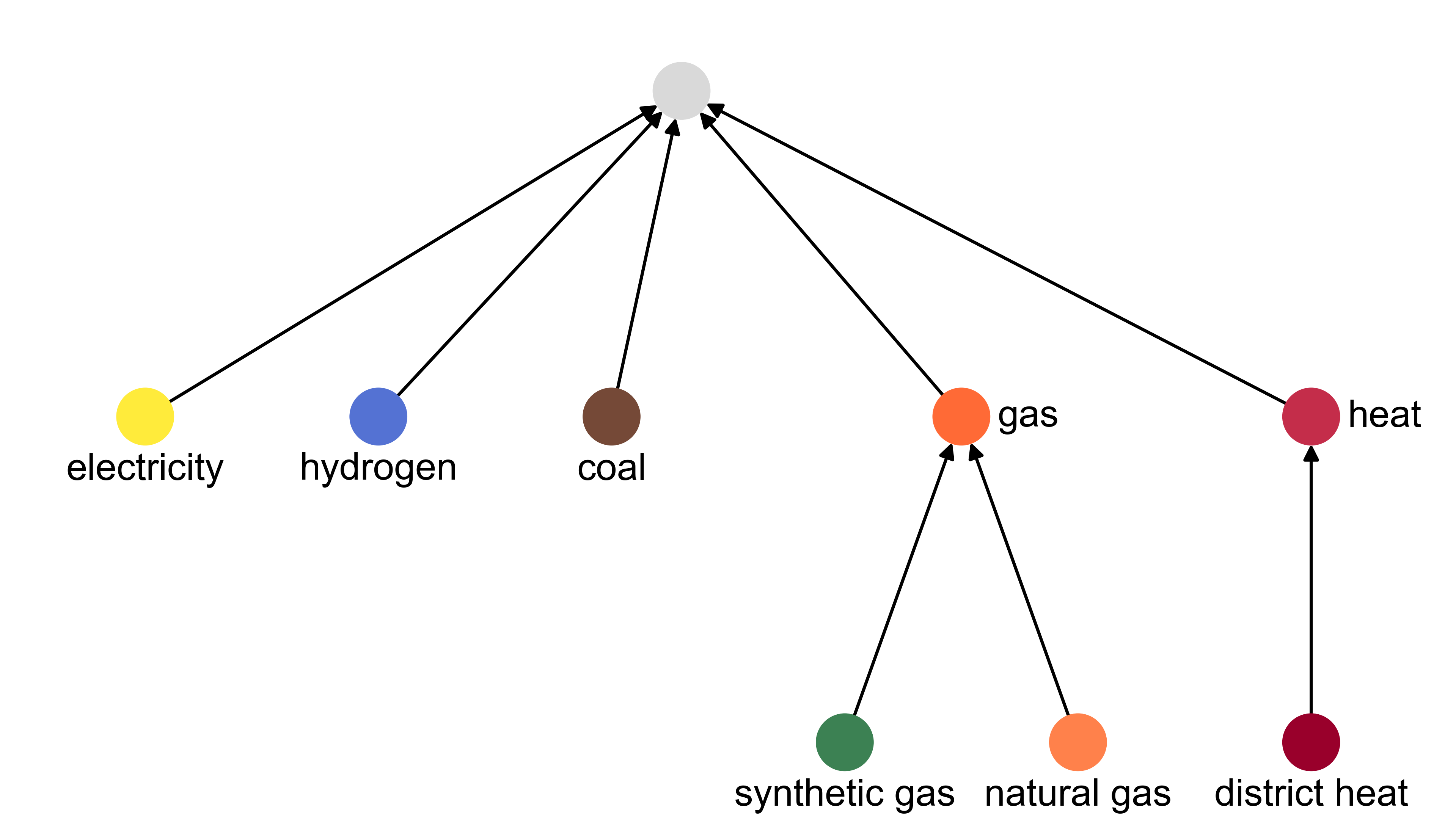
The plotTree function is used to plot the hierarchical trees of sets as introduced in Sets and Mappings.

plotTree(tree_sym::Symbol, model_object::anyModel)

The input tree_sym indicates which set should be plotted (:region,:timestep,:carrier, or :technology). As an example, the tree for :carrier from the demo problem is plotted below.

Optional arguments include:

argument	explanation	default
`plotSize`	length and width of the plot in inches	`(8.0,4.5)`
`fontSize`	font size of labels in plot	`12`
`useColor`	if `true`, tries to obtain node specific colors, otherwise the same color is used for all nodes	`true`
`wide`	controls ratio of horizontal distances between nodes that are on the same level, but have different ancestors (e.g. distance between 'synthetic gas' and 'natural gas' relative to distance between 'natural gas' and 'district heat') first element of input array refers to ratio on the first level and so on	`fill(1.0,30)`

Energy flow

The plotEnergyFlow function provides two ways to visualize the flow of energy within a model: Either as a qualitative node graph or as a quantitative Sankey diagram.

Node graph

To plot a qualitative node graph use the plotEnergyFlow command with the :graph argument.

plotEnergyFlow(:graph, model_object::anyModel)

Nodes either correspond to technologies (grey dots) or energy carriers (colored squares). Edges between technology and energy carrier nodes indicate the carrier is either an input (entering edge) or an output (leaving edge) of the respective technology. Edges between carriers result from inheritance relationships between carriers. These are included, because, according to AnyMOD's graph-based approach, descendants can satisfy the demand for an ancestral carrier (see Göke (2020) for details).

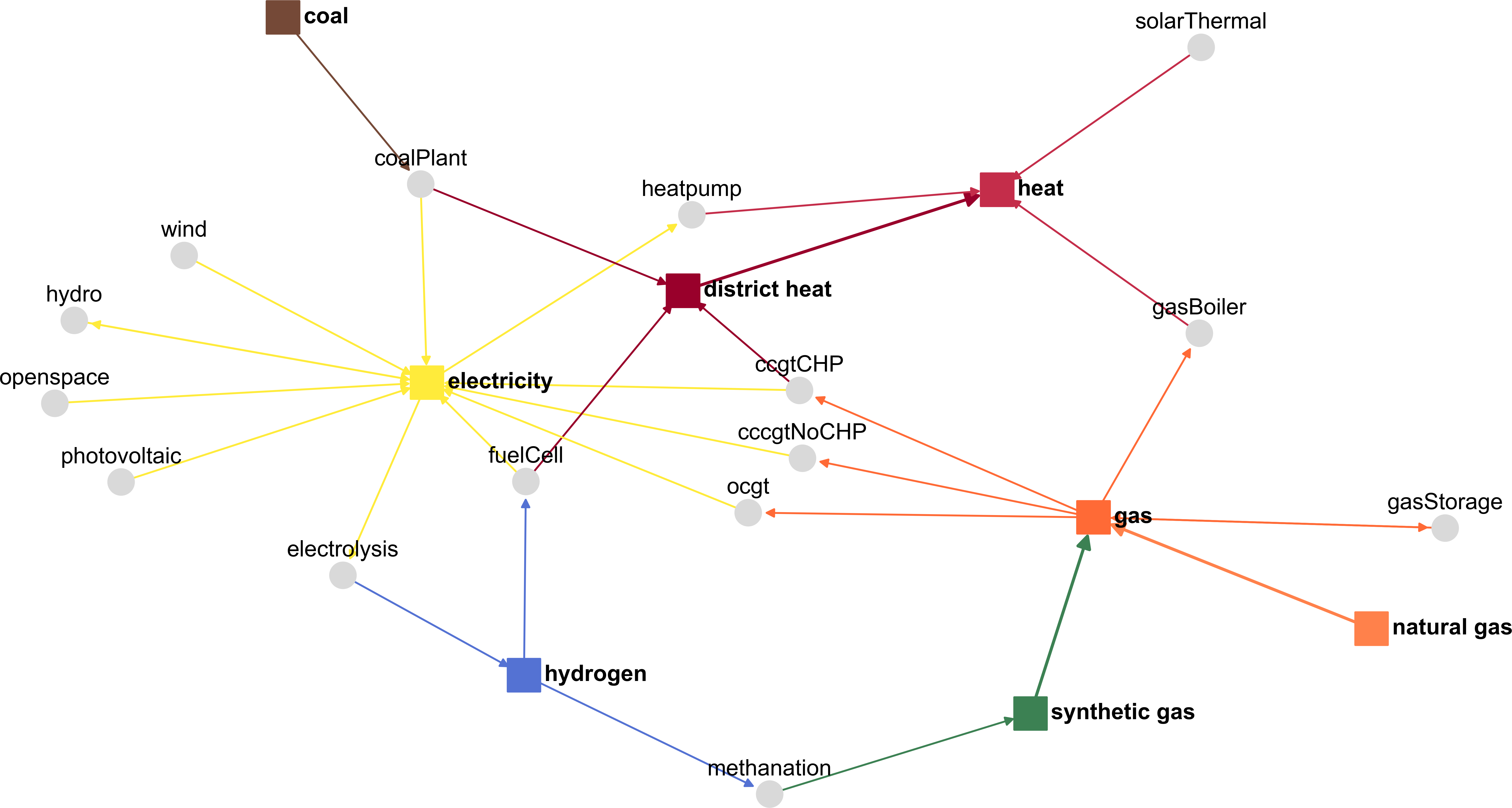
The layout of the graph is created using a force-directed drawing algorithm originally implemented in GraphLayout.jl.

In many cases the resulting layout will be sufficient to get an overview of energy flows for debugging, but inadequate for publication. For this reason, the moveNode! function can be used to adjust the layout.

moveNode!(model_object::anyModel, newPos_arr::Array{Tuple{String,Array{Float64,1}},1})

moveNode! requires an initial layout within that specific nodes are moved. In the example below, an initial layout is created by calling plotEnergyFlow. Afterwards, the node for 'ocgt' is moved 0.2 units to the right and 0.1 units up. The node for 'coal' is moved accordingly. Afterwards, the graph is plotted again with the new layout.

plotEnergyFlow(:graph, model_object)
moveNode!(model_object, [("ocgt",[0.2,0.1]),("coal",[0.15,0.0])])
plotEnergyFlow(:graph, model_object, replot = false)

When plotting again, it is important to set the optional replot argument to false. Otherwise, the original layout algorithm will be run again and overwrite any changes made manually.

Optional arguments for plotting the qualitative node graph are listed below:

argument	explanation	default
`plotSize`	length and width of the plot in inches	`(16.0,9.0)`
`fontSize`	font size of labels in plot	`12`
`useTeColor`	if `true`, tries to obtain node specific colors for technologies, otherwise technology nodes are displayed in grey	`false`
`replot`	if `false`, the current layout of the plot is used instead of computing a new one	`true`
`scaDist`	control parameters for the graph's layout algorithm (see spring.jl for original implementation)	`0.5`
`maxIter`		`5000`
`initTemp`		`2.0`

Sankey diagram

To plot the qualitative energy flows for a solved model use plotEnergyFlow command with the :sankey argument:

plotEnergyFlow(:sankey, model_object::anyModel)

The command will create an entire html application including a dropdown menu and drag-and-drop capabilities. Below is a screenshot of one graph from the solved demo problem.

Optional arguments for plotting a Sankey diagram are:

argument	explanation	default
`plotSize`	length and width of the plot in inches	`(16.0,9.0)`
`minVal`	threshold for energy flows being plotted	`0.1`
`filterFunc`	function to filter certain carriers and technologies from graph for example `x -> x.C == 1` will only include flows associated to the energy carrier with id 1 (see documentation of `tree objects` on how to obtain ids)	`x -> true`
`dropDown`	for each relevant set of the dimensions specified here separate diagrams are created, sets then appear in the dropdown menu within the html output for example `dropDown = (:timestep)` will create diagrams aggregating values across all regions, instead of creating a separate diagram for each region	`(:region,:timestep)`
`rmvNode`	removes specified nodes from the Sankey diagram removal is only possible for nodes that either only have an in- or outgoing flow or exactly one in- and exactly one outgoing flow of equal size in the diagram above for instance, the nodes for 'district heat' or 'curtailment' could be removed, but not for 'ocgt'	`tuple()`
`useTeColor`	if `true`, tries to obtain node specific colors for technologies, otherwise technology nodes are displayed in grey	`true`

Styling

The colors and labels of nodes within plots can be adjusted using the graInfo field of the model object.

The sub-field graInfo.names provides a dictionary that maps node names as specified in the input files to node labels used for plotting. By default, some names occurring in the demo problem are already assigned labels within the dictionary.

Analogously, graInfo.colors assigns colors used for plotting to nodes. Both the actual node name or an assigned label can serve as a key. The assigned value is a tuple of three numbers between 0 and 1 corresponding to a RGB color code.