AnyMOD
AnyMOD.jl is a Julia framework for creating large scale energy system models with multiple periods of capacity expansion formulated as linear optimization problems. It was developed to address the challenges in modelling high-levels of intermittent generation and sectoral integration. A comprehensive description of the framework's graph based methodology can found in the working paper Göke (2020), AnyMOD - A graph-based framework for energy system modelling with high levels of renewables and sector integration. The software itself is seperately introduced in Göke (2020), AnyMOD.jl: A Julia package for creating energy system models.
AnyMODs key characteristic is that all sets (time-steps, regions, energy carriers, and technologies) are organized within a hierarchical tree structure. This enables two unique features:
- The level of temporal and spatial granularity can be varied by energy carrier. For instance, electricity can be modeled with hourly resolution, while supply and demand of gas is balanced daily. As a result, a substantial decrease of computational effort can be achieved. In addition, flexibility inherent to the system, for example in the gas network, can be accounted for.
- The degree to which energy carriers are substitutable when converted, stored, transported, or consumed can be modeled to achieve a detailed but flexible representation of sector integration. As an example, residential and district heat can both equally satisfy heat demand, but technologies to produce these carriers are different.
The framework uses DataFrames to store model elements and relies on JuMP as a back-end. In addition, Julia's multi-threading capabilities are heavily deployed to increase performance. Since models entirely consist of .csv files, they can be developed open and collaboratively using version control (see Model repositories for examples).
Installation
The current version of AnyMOD was developed for Julia 1.3.1. AnyMOD is installed by switching into Julia's package mode by typing ] into the console and then execute add AnyMOD.
Getting started
To introduce the packages’ workflow and core functions, a small-scale example model is created, solved and analyzed. The files of this model can either be found in the installation directory of the package (user/.julia/packages/AnyMOD/.../examples) or manually loaded from the GitHub repository.
Before we can start working with AnyMOD, it needs to be imported via the using command. Afterwards, the function anyModel constructs an AnyMOD model object by reading in the .csv files found within the directory specified by the first argument. The second argument specifies a directory all model outputs are written to. Furthermore, default model options can be overwritten via optional arguments. In this case, the optional argument objName is used to name the model "demo". This name will appear during reporting and added to each output file. The optional argument shortExp defines the span of year between different time-steps of capacity expansion.
using AnyMOD
model_object = anyModel("../demo","results", objName = "demo", shortExp = 10)
During the construction process, all input files are read-in and checked for errors. Afterwards sets are mapped to each other and parameter data is assigned to the different model parts. During the whole process status updates are printed to the console and comprehensive reports are written to a dedicated .csv file. Since after construction, all qualitative model information, meaning all sets and their interrelations, is written, several graphs describing a models´ structure can be plotted.
plotTree(:region, model_object)
plotTree(:carrier, model_object)
plotTree(:technology, model_object, plotSize = (28.0,5.0))
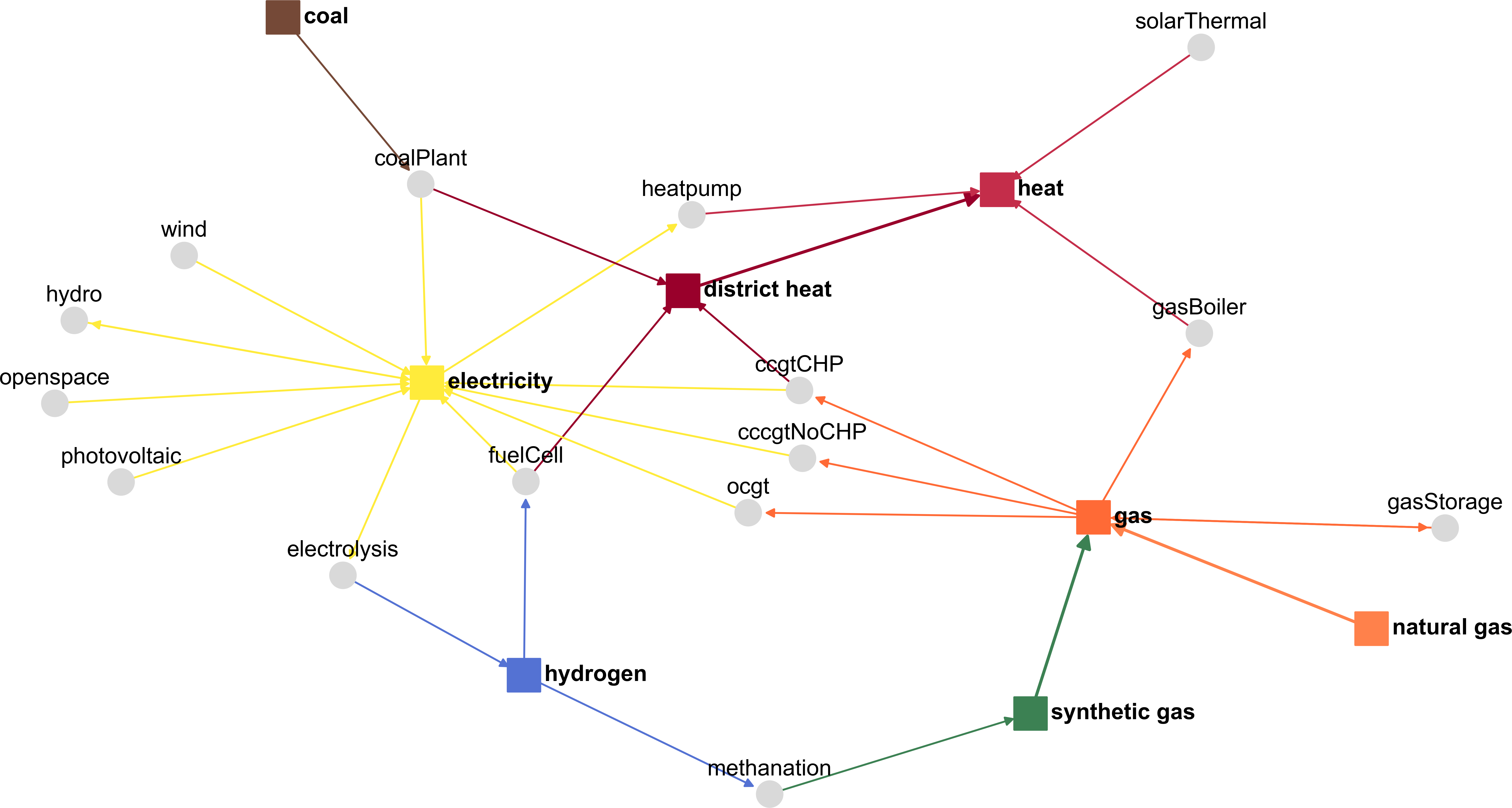
plotEnergyFlow(:graph, model_object)All of these plots will be written to the specified results folder. The first three graphs plotted by plotTree show the rooted tree defining the sets of regions, carriers, and technologies, respectively. As an example, the rooted tree for carriers is displayed below.
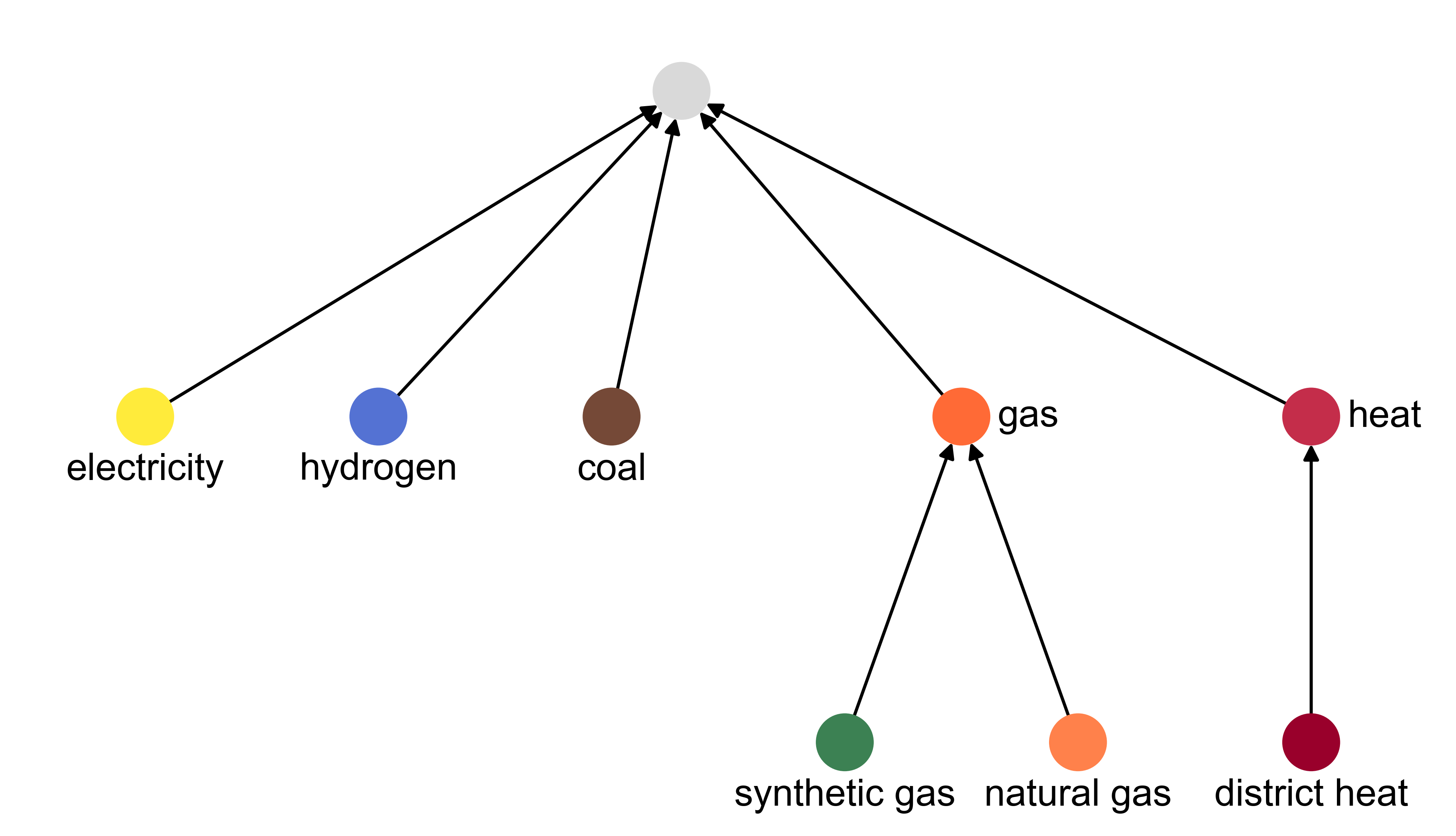
The fourth graph created by using plotEnergyFlow with keyword :graph gives a qualitative overview of all energy flows within a model. Nodes either correspond to technologies (grey dots) or energy carriers (colored squares). Edges between technology and energy carrier nodes indicate the carrier is either an input (entering edge) or an output (leaving edge) of the respective technology. Edges between carriers indicate the same relationships as displayed in the tree above.
To create the variables and constraints of the model's underlying optimization problem, the model object is passed to the createOptModel! function. Afterwards, the setObjective! function is used to set the objective function for optimizing. The function requires a keyword input to indicate what is optimized, but so far only :costs has been implemented. Again, updates and reports are written to the console and to a dedicated reporting file.
createOptModel!(model_object)
setObjective!(:costs, model_object)
To actually solve the created optimization problem, the field of the model structure containing the corresponding JuMP object is passed to the functions of the JuMP package used for this purpose. The JuMP package itself is part of AnyMOD’s dependencies and therefore does not have to be added separately, but the solver does. In this case we used Gurobi, but CPLEX or a non-commercial solver could have been used as well.
using Gurobi
set_optimizer(model_object.optModel, Gurobi.Optimizer)
optimize!(model_object.optModel)
Once a model is solved, results can be obtained and analyzed by the following functions:
reportResults(:summary, model_object)
reportTimeSeries(:electricity, model_object)
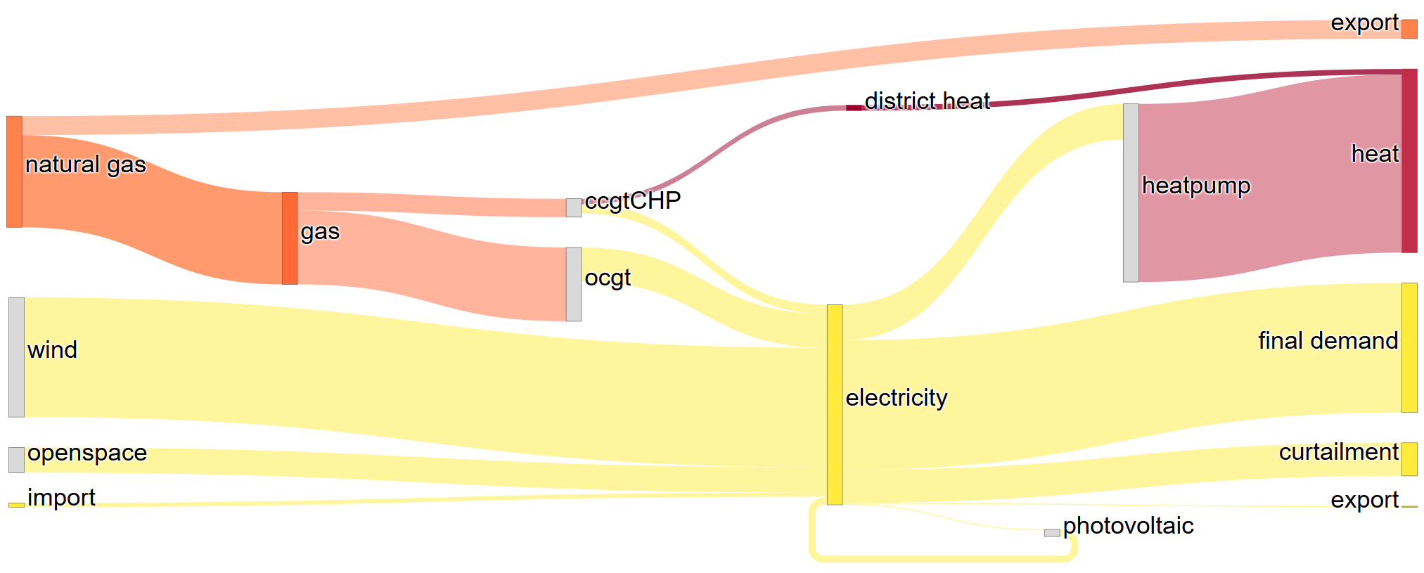
plotEnergyFlow(:sankey, model_object)Depending on the keyword provided, reportResults writes aggregated results to a csv file. :summary gives an overview of installed capacities and yearly use and generation of energy carriers. Other keywords available are :costs and :exchange. reportTimeSeries will write the energy balance and the value of each term within the energy balance of the carrier provided as a keyword. Finally, plotEnergyFlow used with the keyword :sankey creates a sankey diagram that visualizes the quantitative energy flows in the solved model.